yablog: python tips: draw gaussian pdf graph with matplotlib

2011/07/14

python tips: draw gaussian pdf graph with matplotlib

ラベル: python, tips

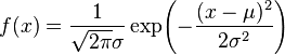
*** Definition of gaussian distribution ***

$f(x)=\frac{1}{\sqrt{2\pi}\sigma} \exp\!\left(-\frac{(x-\mu)^2}{2\sigma^2} \right)$

*** Sample code for drawing gaussian distribution ***

#!/usr/bin/env python                                                           
#coding:utf-8                                                                   

import pylab as pl
import numpy as np
from enthought.mayavi import mlab

def gauss2d(x):
    return 1/np.sqrt(2*np.pi) * np.exp(-(x**2)/2)

def gauss3d(x, y):
    return 1/np.sqrt(2*np.pi) * np.exp(-(x**2 + y**2)/2)

def plot_gauss2d():
    x = np.mgrid[-4:4:100j]

    # matplotlib functions                                                      
    pl.plot(gauss2d(x), 'bo-')
    pl.ylabel('gauss2d(x)')
    pl.xlabel('x')
    pl.show()

def plot_gauss3d():
    x, y = np.mgrid[-4:4:100j, -4:4:100j]
    """                                                                         
    x, y = np.mgrid[-2:2:5j, -2:2:5j]                                           
    array([[[-2., -2., -2., -2., -2.],                                          
            [-1., -1., -1., -1., -1.],                                          
            [ 0.,  0.,  0.,  0.,  0.],                                          
            [ 1.,  1.,  1.,  1.,  1.],                                          
            [ 2.,  2.,  2.,  2.,  2.]],                                         
           [[-2., -1.,  0.,  1.,  2.],                                          
            [-2., -1.,  0.,  1.,  2.],                                          
            [-2., -1.,  0.,  1.,  2.],                                          
            [-2., -1.,  0.,  1.,  2.],                                          
            [-2., -1.,  0.,  1.,  2.]]])                                        
    x[0,0] ==> -2.0                                                             
    y[0,0] ==> -2.0                                                             
    """

    # matplotlib functions                                                      
    pl.plot(gauss3d(x, y))
    pl.ylabel('gauss3d(x)')
    pl.xlabel('x')
    pl.show()

def plot_gauss3d_mayavi():
    x, y = np.mgrid[-4:4:100j, -4:4:100j]
    z = gauss3d(x, y)

    mlab.surf(z, warp_scale='auto')
    mlab.outline()
    mlab.axes()
    mlab.show()

def main():
    #plot_gauss2d()                                                             
    #plot_gauss3d()                                                             
    plot_gauss3d_mayavi()

if __name__ == "__main__":
    main()